译者:hxhgxy 来源:http://blogs.msdn.com/excel
发表于:2006年7月7日
PivotTables 12: Filtering OLAP data, and some “persistence” improvements
数据透视表 12:筛选OLAP数据,以及一些“持续”改进
In a previous post I covered the new sorting and filtering capabilities of Excel 12 PivotTables. Those features are available for any PivotTable, regardless of the data source. There are a few additional filtering options available for PivotTables connected to Analysis Services, so I want to review those today. I also wanted to make a short point about some “formatting persistence” work we have done in Excel 12.
在前面的文章中,我讲过了Excel 12数据透视表的新排序和筛选功能。这些功能可为任何数据透视表所用,不管是什么数据源。连接到Analysis Services的数据透视表还有一些额外的筛选选项,因此今天我想要回顾一下这些。我也想要简短地看一下我们在Excel 12里所作的“格式持续性”的工作。
Filtering by member properties
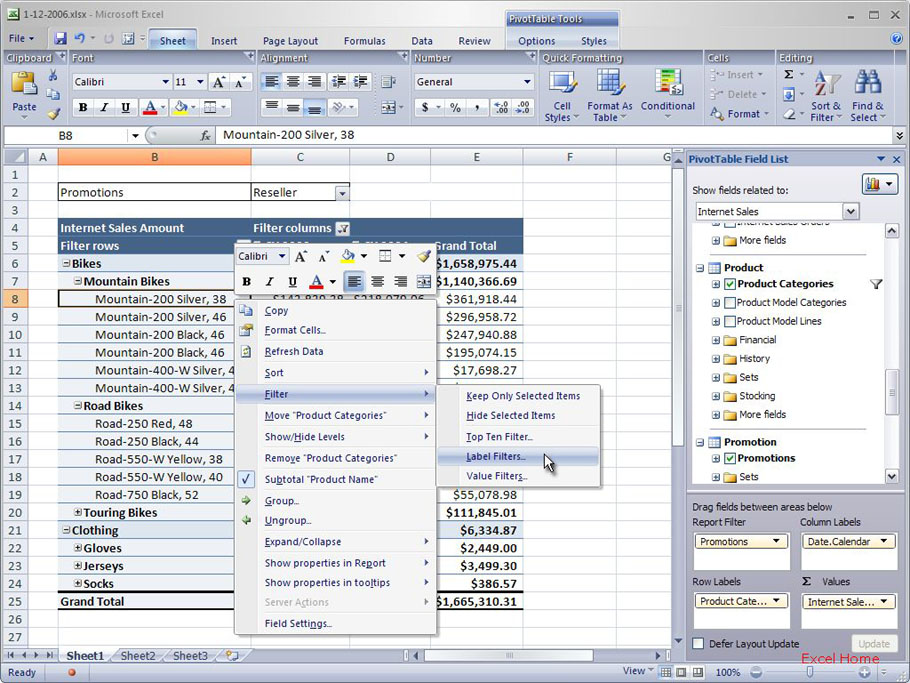
A few days ago I wrote about member properties. When a PivotTable is connected to data from Analysis Services, you can filter items in the PivotTable based on the value of that item’s member properties. Let’s look at an example. In the screenshot below, I have a PivotTable with Product Categories, Products, and Sales Amounts. I might want to filter the Products in the PivotTable by one of their properties. I can do this by applying a Label Filter … I simply need to right-click on one of the products and choose Filter|Label Filer from the context menu.
筛选成员属性
几天前,我写了关于成员属性的一些东西。当数据透视表从Analysis Services连接到数据时,你可以基于那些项目的属性值筛选项目。我们来看一个示例。在下面的截屏中,我有一个数据透视表,有Product Categories(产品品类), Products(产品)和Sales Amounts(销售数量)。我可能想要通过它们的某个属性在数据透视表里筛选Products。我可以通过申请一个Label Filter实现它……我只是简单地在某个产品上单击右键,并且从快捷菜单上选择Filter | Label Filter(译者,原文误为Filer)。
(Click to enlarge)
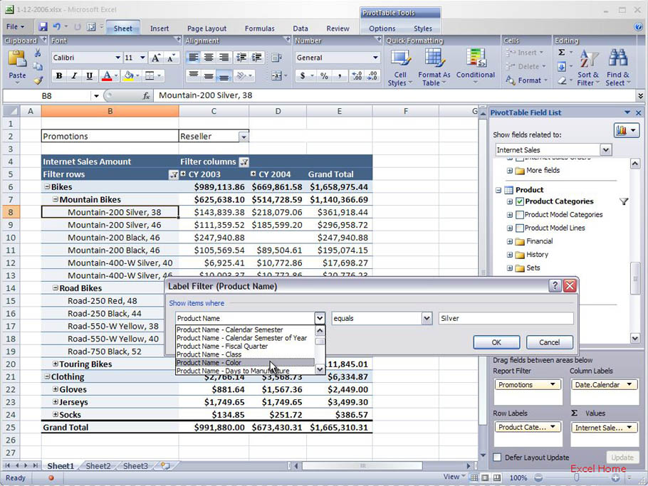
This brings up the Label Filter dialog. Since there are member properties defined for the field I selected, the Label Filter dialog lists those for me to select from.
这会打开Label Filter对话框。因为我所选择的字段已经定义了很多成员属性,Label Filter对话框将它们列出供我从中选择。
(Click to enlarge)
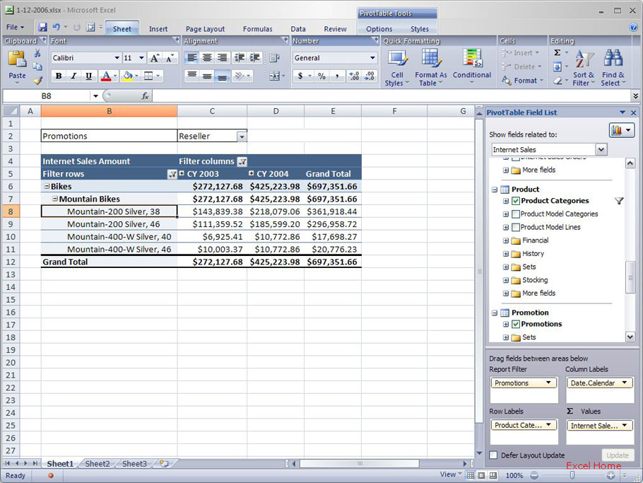
If I pick the field name (“Product Name” in the example), the filter will be applied to the visible items in the PivotTable. If I pick one of the member properties, however, which are listed under the field name in the drop down, the filter will look at the member-property values instead. If I only want to see the bikes where the color is silver, I can use the Colour member property to do that. Here is a screenshot of the PivotTable filtered by the color member property so only silver bikes are displayed.
如果选择字段名称(本例中是“Product Name”),该筛选就会应用数据透视表中可见的项目。然而,如果我选择了某个列在字段名称下面下拉框里的成员属性,筛选器就会只关注该成员属性值。如果我只想看看银色的自行车的话,那么我可以使用Colour成员属性来实现。这里有个截屏,用颜色成员属性筛选的数据透视表,因此只有银色的自行车被显示了。
(Click to enlarge)
Filtering by values not displayed in the PivotTable
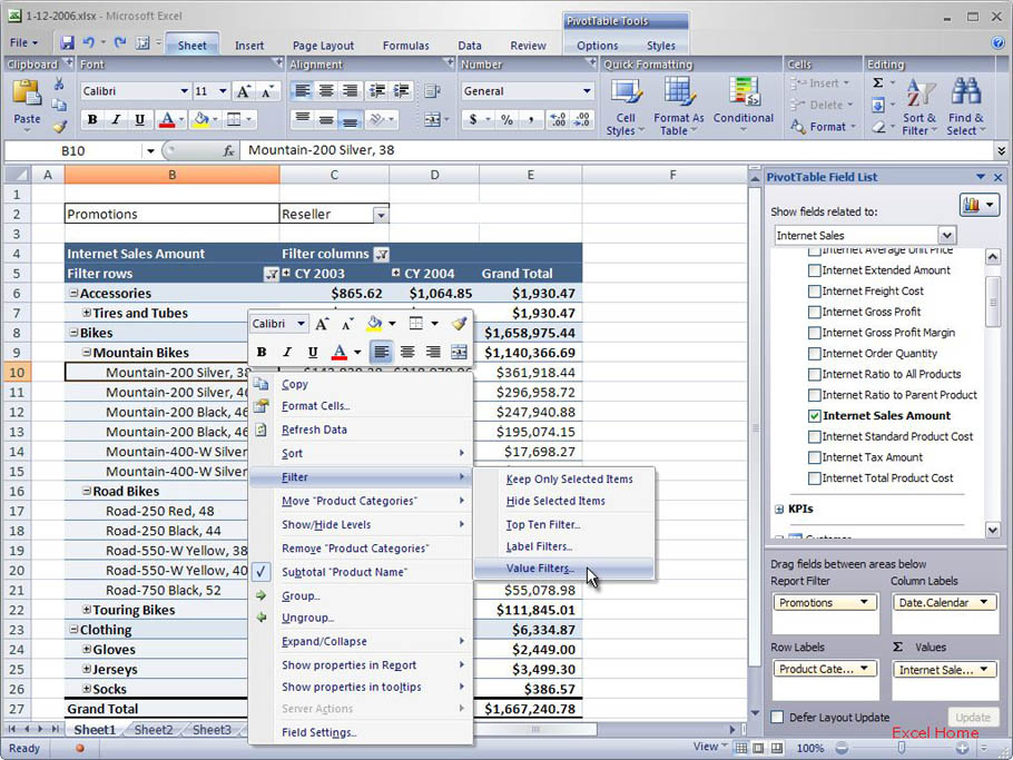
Another filter ability specific to PivotTables connected to Analysis Server is the ability to filter items by a value that is not currently displayed in the PivotTable. For example, you might want to filter products in a sales report by the profit margin of each product, even though profit is not showing in the PivotTable. Again, let’s walk through an example. Below is a PivotTable that shows Sales Amount by Product and Product Category. In this case, I only want to see products that have a profit margin which is greater than 40%. To do this I’ll apply a value filter to my PivotTable.
筛选没有显示在数据透视表里的数值
连接到Analysis Server的数据透视表的另外一个筛选功能是筛选当前并没有显示在该数据透视表里的数值。例如,你可能想要在一个销售报表中,通过每个产品的利润来筛选产品,尽管利润没有显示在该数据透视表里。同样,我们来看一个例子。下面是个按产品和产品品类显示销售量的数据透视表。在本示例中,我仅想要查看利润超过40%的产品。为了做到这样,我将应用一个数值筛选到我的数据透视表。
(Click to enlarge)
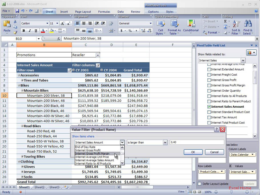
After I select Value Filter from the context menu, I see the Value Filter dialog. When I drop the first drop-down, all the different value fields available are listed, even though the PivotTable only contains Sales Amount. I simply select Gross Profit Margin, type in 40, and press OK.
我在快捷菜单中选择Value Filter后,我看到Value Filter对话框。当我拉下第一个下拉列表时,列出了所有可用的不同数值字段,尽管该数据透视表仅包含Sales Amount(销售量)。我只是简单地选择了Gross Profit Margin,输入40,并按下OK。
(Click to enlarge)