译者:hxhgxy 来源:http://blogs.msdn.com/excel
发表于:2006年7月7日
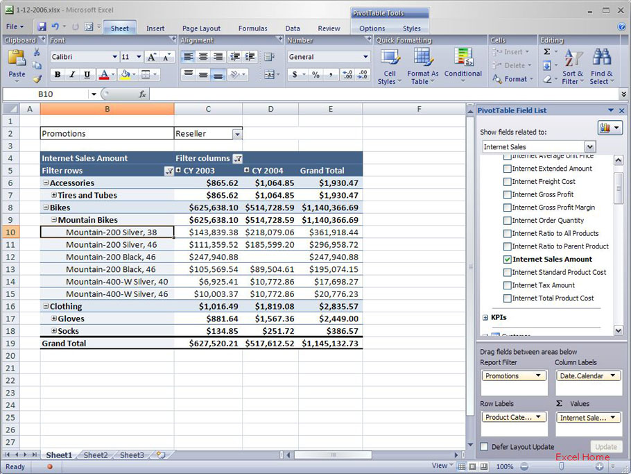
And now my report is showing only bikes with a profit margin greater than 40%.
现在报表只显示利润大于40%的自行车了。
(Click to enlarge)
I am personally a very big fan of this feature.
我个人认为这个功能非常有趣。
Hiding levels of hierarchies
Excel 12 PivotTables that are connected to Analysis Services allow you to hide any level of a hierarchy as long as at least one level is still visible. As an example, say I want to compare bikes independent of what type of bike they are (I don’t want to see Category or Subcategory information). To do this, I can hide the parent levels of the product name level. Specifically, I just need to select Show/Hide Levels from the PivotTable context menu, and from there I can toggle on or off any levels I like.
隐藏层次级别
连接到Analysis Services的Excel 12数据透视表允许你隐藏任何层次级,只要至少还有一级是可见的就可以。举例说,假如我想比较自行车,不管它们是什么型号(我不要查看Category或Subcategory信息)。要实现这个,我可以隐藏产品名称级别的父级别。确切地说,我只需要从数据透视表的右键菜单中选择显示、隐藏就可以,并且从那里,我可以切换任意级别的开或关。

(Click to enlarge)
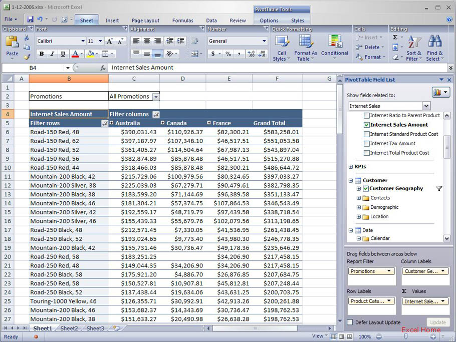
After hiding the two levels, I’ve also sorted the bikes by their individual total sales amounts and, as you can see in the screenshot below, I can now work with the bikes across their groups. Notice that mountain bikes are now mixed with road bikes etc.
在隐藏两级后,我也按它们的销售量进行自行车排序,如你在下面截屏看到的,我现在可以在自行车组合里查看它们了。注意现在山地自行车和道路自行车等是混在一起的。
(Click to enlarge)
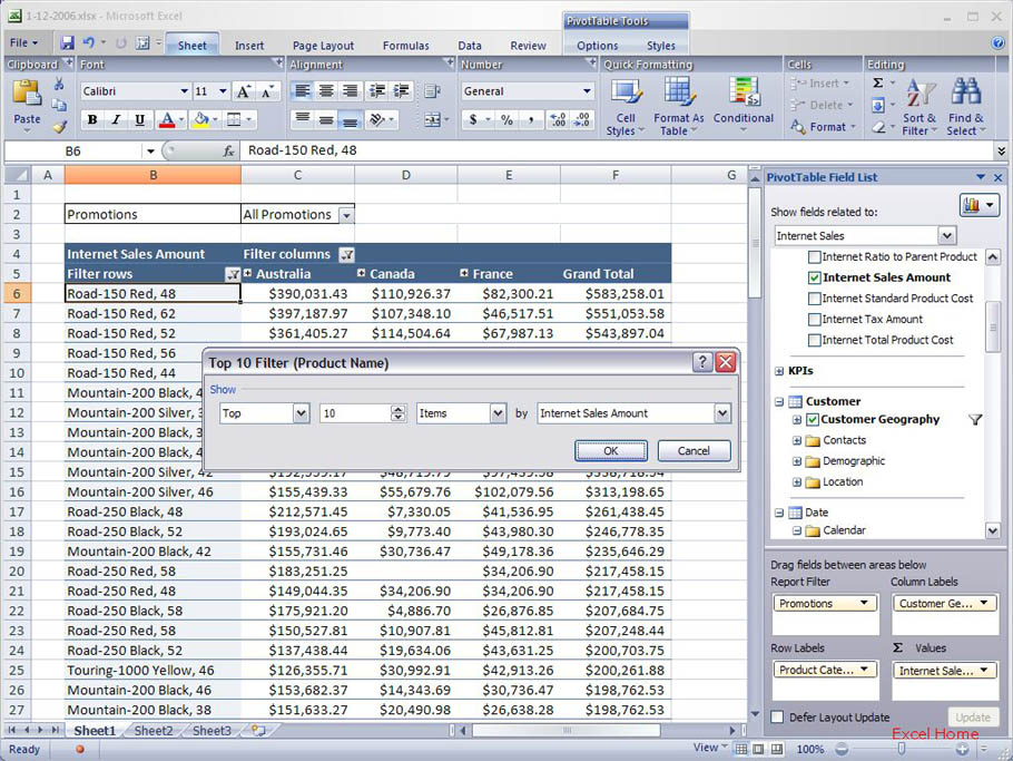
This also allows me to produce, for example, a “Top 10” list of the best-selling bikes regardless of category. This is another example of the very powerful analysis capabilities available in Excel 12 PivotTables.
例如,这也允许我创建一个“前十位”销售最好的自行车,不管其品类。这是Excel 12数据透视表拥有强大分析能力的另一个例子。
(Click to enlarge)
Here is the final result.
这是最终结果。

(Click to enlarge)
If I now unhide the Subcategory level, the filter will be reevaluated in the new context, and I will get a “Top 10” list of bikes for each subcategory. I think that’s pretty neat too.
如果我现在取消隐藏的Subcategory级的话,筛选会重新评估新的上下文,并且会获得每个子品类中的“前十位”的自行车清单。我认为那也是很灵巧的。
Better persistence of user applied formatting
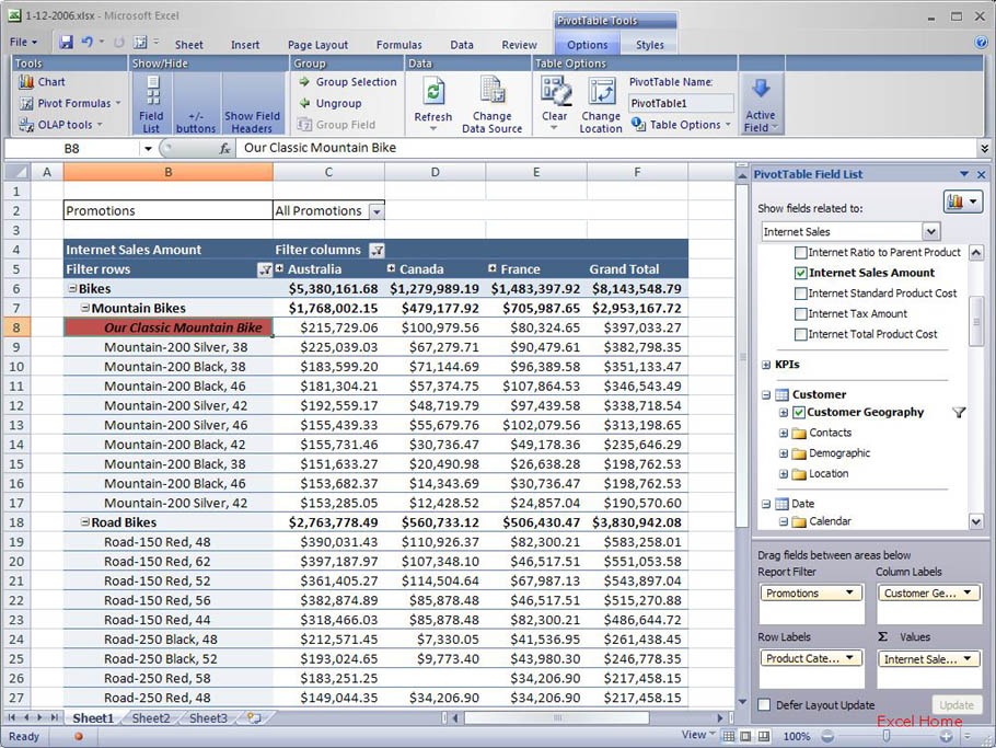
Finally, we have improved the persistence of user-applied formatting in OLAP PivotTables. The screenshot below shows a PivotTable where I’ve manually change the name of a bike to “Our Classic Mountain Bike” by typing the new name into the cell, and where I have also made the text bold + italics and then set the cell background color to red.
用户应用格式的持续性更好了
最后,我们改进了OLAP数据透视表的用户应用格式的持续性。下面的截屏显示一个数据透视表,我通过在单元格里输入新名称,手动更改一自行车的名称为“Our Classic Mountain Bike”,并且将文本设置为粗斜体,然后设置单元格背景颜色为红色。
(Click to enlarge)
Now, if I collapse Mountain Bikes in the PivotTable (which hides the individual mountain bikes), and then expand Mountain Bikes again, the mountain bike I formatted will still be formatted exactly like before I collapsed Mountain Bikes. In current versions of Excel, all the formatting is lost in this scenario. A small item, but one I am sure folks will be glad to see “fixed.”
现在。如果我折叠数据透视表里的山地自行车(隐藏该具体的山地自行车),然后在展开山地自行车,我设置了格式的那个山地自行车将仍然会象我折叠山地自行车之前那样完成一样的格式。在现在的Excel版本中,在这样的方案中,所有的格式都会丢失。一个很小的项目,但是我肯定人们会喜欢看到它“固定了”。
Published Thursday, January 12, 2006 8:24 PM by David Gainer
注:本文翻译自http://blogs.msdn.com/excel,原文作者为David Gainer(a Microsoft employee),Excel home授权转载。严禁任何人以任何形式转载,违者必究。