译者:taller 来源:http://blogs.msdn.com/excel
发表于:2006年7月7日
Tables Part 2: Stickiness, Structured Selection, And More
列表(第二部分):附着,结构化选中…
(译者注:本文中的“附着”是原文中“Stickinees”或者“Stick”的直译)
One of the key benefits of tables is how other features in Excel 12 behave more predictably and more like you would expect when a table is present. This is made possible by the fact that Excel knows exactly where the table starts and ends, where the header row is, which cells make up the data and which columns they belong to, where the total row is, etc. So how exactly does this benefit the user? Here are some of the different ways in Excel’s awareness of the structure of your data changes the user experience.
Excel 12列表的一个核心优点在于-当使用列表时,其他相关功能能够更有预测性的迎合用户的需求,为了使这一切成为可能,Excel必须准确定知道列表的相关信息,如:开始和结束位置以及标题行位置,哪些单元格包含数据,它们分别属于哪些列等等。那么这些功能到底对终端用户有什么好处呢?Excel所具有的识别用户数据结构的不同方式可以带给用户不同以往的感受。
Stickiness
附着
When a user does something to a column of data in a table, it “sticks”. What exactly does that mean? If, for example, a user applies a conditional format to an entire column of a table, Excel assumes that the conditional format is always meant to cover the entire table column. So as new rows are added to the table, either in the middle or at the end, and as rows are deleted, Excel will automatically extend or contract the conditional formatting rule appropriately. The rule “sticks” to the column. We already saw this with the example in my previous post, but it doesn’t just stop with conditional formatting. This concept works with just about anything you can apply to a column, such as formatting (anything in the Format Cells dialog), cell protection, data validation, etc. In addition, this behaviour also applies to anything that holds on to a reference, such as formulas, charts and PivotTables.
当用户对列表的某列进行操作时,其相关的属性将被“附着”,这究竟是什么意思呢?例如用户在列表的某列使用了条件格式,Excel就会假定条件格式会永远应用到该列,所以无论是在列表的中间还是最后添加或者删除行时,Excel会相应地扩展或者收缩条件格式的范围及其相关的规则,如格式(单元格格式对话框中的所有选项)、单元格保护、数据有效性等,将“附着”在该列,另外,这种方式会应用在任何与引用相关的功能,例如公式、表格和数据透视表。
How do you make something “sticky”? There’s no explicit gesture for this. Excel just assumes that anytime something is done to an entire column, the setting is meant to always follow the column. So, if a user selects a table column and applies a data validation rule, that rule will grow and shrink with the table. Create a PivotTable that uses a table as its data source, and that Pivot Table will automatically pick up new rows from the table. Ditto for charts. To be precise, when I say “entire column” in this context, I really mean all the data rows. It is not necessary to also include the header cell – this way you don’t have to include the header in order to, for example, make the “currency” number format stick to a column for example.
那么,我们如何使某些功能“附着”哪?到目前为止我们没有任何方法可以定制它。Excel只是假设任何时候对于整列进行的设置,将永远跟随本列,如果用户选择列表的某列设置数据有效性,那么数据有效性的范围会随着列表而扩大或者收缩,如果设置列表为数据透视表的数据源,那么列表新增加的数据将自动添加到数据透视表中,图表具备同样的功能。准确的说,本文中所提及的“整列”是指包含列表中所有行的数据,但是标题行的数据不一定包含在内,
This stickiness also applies to new columns. For example, if a table is used as the data source for a chart, then any new columns I add to the table will get picked up by the chart. In addition, properties set on the entire table, headers, and the total row (more on what a total row is in a later post) are also “sticky”.
附着功能同样会应用到新增加的列,例如:一个列表作为图表的数据源,列表增加列时会自动更新图表,另外,整个表格的所有属性、标题和汇总(以后的帖子中会更多的阐述汇总)也会相应的“附着”。
Selection
选中
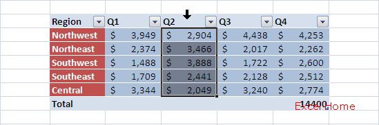
Now that Excel recognizes things like rows and columns in my tables, it is only natural that it provide simple ways to select those elements of a table. A single mouse click can select one or more rows, one or more columns, or the entire table. To select a column in a table, simply hover the mouse over the top of the header until the mouse cursor turns into a down-arrow and click.
现在Excel可以识别列表中的某些元素,如行和列,利用简单的方法选中这些元素就成为一个自然的需求,通过简单点击一次鼠标就可以选中一行或者多行、一列或者多列,乃至整个列表,如果希望选中列表的某列,只需要将鼠标移到标题行之上,当鼠标变成下箭头时点击鼠标就可以完成。
To select a row, hover the mouse over to the left edge of a row until the mouse cursor turns into a right-arrow and click. And to select the entire table, hover the mouse over the top-left corner of the table until you see an arrow that points down and right and click.
如果希望选中列表的某行,只需要将鼠标移到列表左侧边界,当鼠标变成右箭头时点击鼠标就可以完成,如果希望选中整个列表,则需要将鼠标移列表的左上角,当鼠标变成向右下方的箭头时点击鼠标就可以完成。
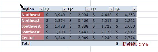
Note that column and table selection have two behaviours. The first click always selects just the data portion of the column/table. This makes it easy to select a column of numbers and apply formatting or other properties to the data in the column. The second click expands the selection to cover everything in the column/table, header and all. This is useful for copy/paste operations or rearranging columns in a table.
注意选中行和列有两种方式,第一次点击总是仅仅选中列表中某列的数据部分,这样可以很容易的选中一列数字,并设置格式或者修改其他属性,第二次点击将选中列表中该列的所有内容,包括标题行在内,这种方式可以用于复制/粘贴或者调整该列在列表中的位置。
If you are a keyboard junkie (like many of the people reading this seem to be), note that there is keyboard support for these selection behaviours. The existing shortcut keys for row and column selection, SHIFT+SPACE and CTRL+SPACE respectively, have been modified to work with tables. For example, pressing CTRL+SPACE once selects all the data rows in a table column. The second press expands the selection to encompass the entire table column, and the third press expands it again to encompass the entire worksheet column.
如果你喜欢使用快捷键(似乎阅读这个帖子的多少人都是这样),使用键盘同样可以实现选中功能,在先前版本中使用的行和列的选择快捷键<SHIFT+SPACE>和<CTRL+SPACE>现在可以仍然可以应用于列表,例如:按一次<CTRL+SPACE>可以选中列表中某列的所有数据,第二次按下快捷键可以列表中该列第所有内容,再次按下快捷键则选中工作表的整列。
What Column am I in again?
再次请问——我在哪列中?
This is one of my favorites. When working with large data sets, it’s easy to scroll the headers off the screen and forget which column you are looking at, especially if many of the columns have similar data in them. Once you have declared something a table in Excel 12, this problem will go away – when navigating a large table and the table’s headers have been scrolled off the screen, Excel will insert the table headers into the sheet header row where the A, B, C headings appear (see the screen shot below). For example, when I scroll this table upwards …
这是我非常喜欢的功能之一,当你处理大量数据时,需要滚动屏幕,标题行时常消失的无影无踪,如果有很多列都有类似的数据,那么用户根本无法记得自己在查看哪列的数据,如果你在Excel 12中使用列表功能,这个问题将不再存在,用户浏览很大的列表时,当列表的标题行将要移出屏幕时,Excel会将系统原来的列标题的A,B,C替换为列表的标题行(请看下面的截屏图),例如当我在不停地滚动屏幕时……
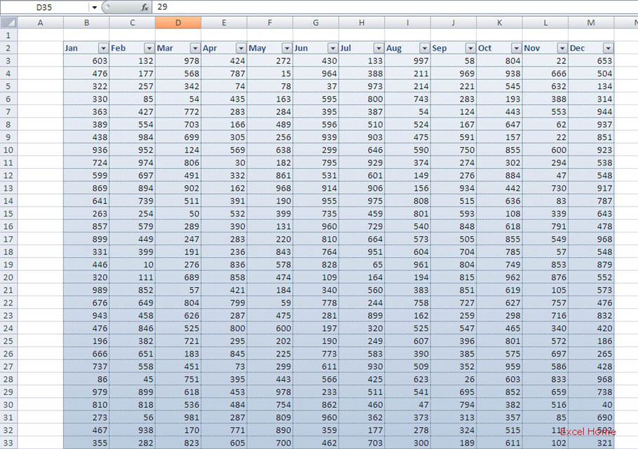
the header text shows up in place of the sheet headers.
……列表的标题行文字显示在工作表列标题的位置。
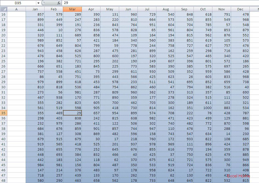
This makes it much easier to keep track of things without having to split screen/freeze panes. Note, the table headers will only be visible as long as the active cell is somewhere inside the table. If you select outside the table, the standard A, B, C headers return.
这样即使不使用分割窗口/冻结功能也能很清楚的知道自己的位置,请注意只有在当前活动单元格位于列表中时,才会显示列表标题,如果选中列表之外的单元格,工作表列标题将恢复原状。
More Conditional Formatting Goodness
条件格式的更多精华
Back at the start of my conditional formatting posts, I said that one of the things we set out to do was to provide a better experience in Tables – lowering the bar for conditional formatting rules that previously required formulas or fiddling. Here are two features we added to conditional formatting when a user is working with a table.
在◎条件格式◎的帖子开始处,我说过我们将要实现的一件事情就是提供更好的列表体验-减少以前设置条件格式时所需要输入的公式或一些无关紧要的东西,我们提供两个新的功能可以应用于列表条件格式。
First, we added a “format entire row” option that appears when defining a conditional format rule on a table.
第一,当设置列表的条件格式时,将会出现“格式化整行”的选项
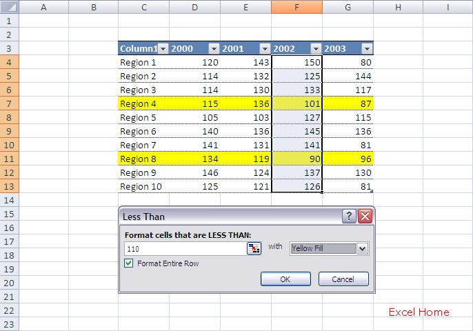
When this option is turned on, the entire table row will be highlighted when a condition is met within a specific column. Achieving this in the past required more advanced knowledge of conditional formatting. Now you can treat it like any simple rule – just select the olumn you are interested in evaluating, and select this option if you want the result to show across the entire row.
如果选中这个选项,当条件满足时,该列表的相应数据行整行都会突出显示,在过去只有具备高超的条件格式应用技巧才能够实现这个效果,现在则变得非常简单,只需要在设置条件格式时选中这个选项,就可以实现整行突出显示的效果。
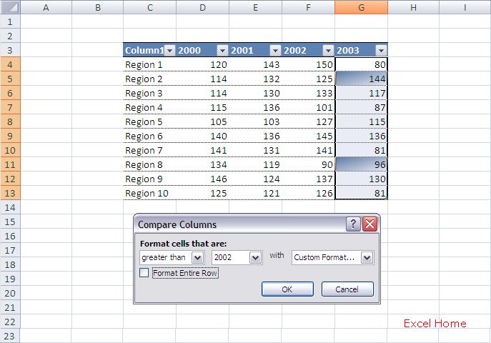
Second, we added a “compare columns” rule to the list of rules available when setting up conditional formatting on tables. This rule allows you to format cells of a table column based on comparisons with values in another column – you can use this, for example, to highlight any rows where the values in the “2005 Profits” column are less than the values in “2004 Profits” column. Again, the fact that Excel knows that there are columns in your table makes it possible to surface very easy UI to quickly set up these sorts of conditions.
第二,我们在列表的条件格式中添加了“对比列”,这可以基于本列和其他列数据的比较来设置格式,例如,突出显示“2005 Profits”少于“2004 Profits”的数据行,正是因为Excel能够识别列表的列,所以我们才能通过简单的用户界面来设置条件。
That’s it for now. In my next table post I’ll go into all the work we’ve done around tables, formulas, and referencing.
今天就到这里,在我的下一个列表的帖子中我将详细阐述列表、公式和引用。
Published Thursday, October 27, 2005 10:42 AM by David Gainer
注:本文翻译自http://blogs.msdn.com/excel ,原文作者为David Gainer(a Microsoft employee),Excel Home 授权转载。严禁任何人以任何形式转载,违者必究。