译者：hxhgxy  来源：http://blogs.msdn.com/excel
发表于：2006年7月7日

PivotTables 11: Key Performance Indicators, Actions, and Named Sets
数据透视表 11：关键性能指标，动作和名称集

Today, I will cover three additional features of Analysis Services that Excel 12 PivotTables support – Key Performance Indicators, Actions, and Named Sets.
今天，我将谈及Excel 12 数据透视表支持的Analysis Services的另外三个特点——关键性能指标，动作和名称集。

Key Performance Indicators
SQL Server Analysis Services 2005 introduced the notion of key performance indicators (KPIs). A KPI is a set of calculations defined in an Analysis Services model that represent key business metrics which can be displayed in reports, portals, dashboards, etc. There is a lot of literature out there on KPIs, so I will not spend a lot of time on the value of KPIs as a concept, but I do want to briefly cover how a KPI is defined in Analysis Services. A KPI has four main components:
关键性能指标
SQL Server Analysis Services 2005引进了关键性能指标（KPIs）的概念。KPI是Analysis Services模型里定义的一套计算，代表可以在报告，入口，仪表板等上面显示的关键业务方法。关于KPIs，有很多著述，因此我不会花很多时间讨论KPIs这个概念，但是我确实想简单地讲讲KPI是如何在Analysis Services里定义的。KPI有四个主要成员：

• Value. The current value of the business metric – this could be a physical measure like Sales, a calculated measure like Profit, or a custom calculation defined specifically in the KPI.
• 数值。业务方法的当前值——这可以是一个具体的衡量如销售，计算的衡量如利润，或者一个在KPI里特别的自定义计算。

• Goal. The target for the business metric – this is usually an MDX expression that resolves to a value.
• 目标。业务方法的目标——这通常是分解为一个数值的MDX表达式。

• Status. A number defining the current status of the Value, normalized in the range -1 (very bad) to +1 (very good) – this is also an MDX expression.
• 现状。一个定义数值当前状态的数字，标准化为范围-1（非常差）到1（非常好）——这也是个MDX表达式。

• Trend. An indication defining how the business metric is developing over time – getting better or worse relative to its goal. Trend is also normalized between -1 and 1, and also an MDX expression.
• 趋势。定义业务方法如何发展的预测——对目标变好或者变坏。趋势也标准化为-1到1，并且也是一个MDX表达式。

In Excel 12, KPIs are listed in the field list in a special KPIs folder. Here is an example of a KPI for Profit Margin.
在Excel 12里，KPIs列在字段清单的一个特殊KPI文件夹里。这里有个Profit Margin的KPI示例。

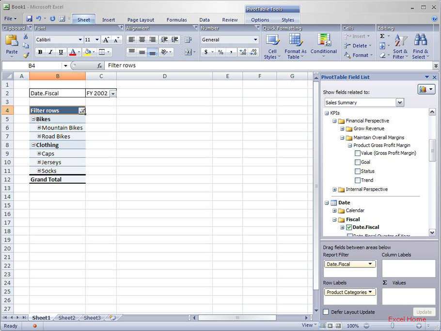
Each KPI component can be added to the PivotTable Values area by checking the checkbox just like any other field. Let’s take a look at an example, specifically, and example of adding Value, Goal, Status, and Trend to a report on our Products and Product Categories. Here is what the report looks like when I add those four components.
每个KPI成员可以通过勾选复选框添加到数据透视表数值区域，正如其它字段一样。我们来看一个例子，一个专门添加数值，目标，现状和趋势到我们产品和产品品类报告中的例子。当我添加这四个成员时，报告就是下面这个样子。

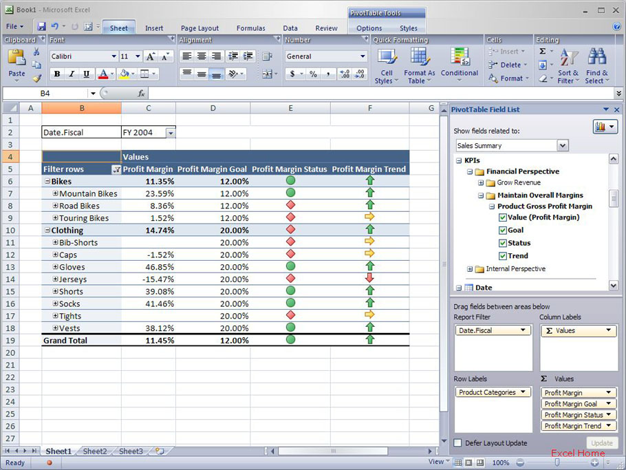
As you can see, Value and Goal are presented as numbers. Status and Trend, on the other hand, are nice graphical representations – they can be used to get a very quick visual overview of your business as it is easy to pick out outliers etc. As I mentioned, Status and Trend are normalized values between -1.0 and 1.0. Since these sorts of numerical values are not very interesting to show in a report, we have worked with the SQL Server Analysis Services 2005 team to develop a set of images to represent the Status and Trend for any KPI. The images to be used are defined in the Analysis Services model, so everyone that looks at the Status or Trend in Excel sees the same graphic. Those of you that remember the conditional formatting post I wrote on Icon Sets have probably already figured out we are using that capability in Excel 12 as part of this KPI feature.
正如你所见，数值和目标用数字表示，另外，现状和趋势是一种美观的图形表示——它们可以给你的业务以非常快捷的视觉效果，非常容易抓住突出者等。正如我提过，现状和趋势通常值在-1到1之间。因为这些数字值显示在报告里不会有什么好奇的，我们和SQL Server Analysis Services 2005开发组合作，开发了一套图形来代表任何KPI的现状和趋势。这些即将使用的图形是在Analysis Services模型里定义的，因此任何从Excel里看到的现状和趋势是同样的图形。你们中有记得我发表的关于图标集的条件格式文章，可能已经领会到我们也使用那种技术在Excel 12里作为一部分KPI特点。

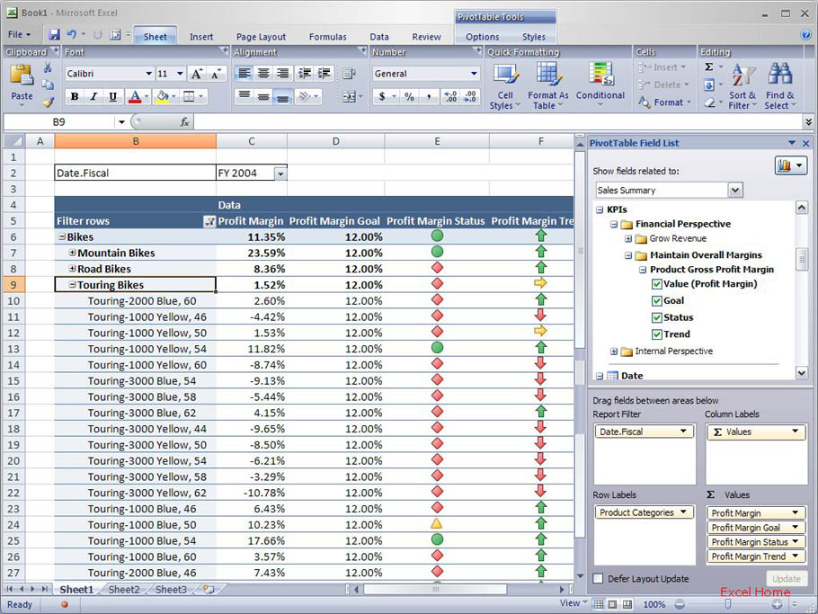
Even better, since this is a PivotTable, as I expand/collapse items in the PivotTable or perform other operations, the KPI components will automatically be calculated in the new context. For example, if I expand “Touring Bikes”, the PivotTable will show the values of the KPI components and update the Status and Trend graphics accordingly.
更妙之处在于，因为这是数据透视表，当我展开、折叠数据透视表里的项目或者执行其它操作是，KPI成员讲会在新下上下文中自动重新计算。例如，如果我展开“Touring Bikes”，数据透视表会显示KPI成员的数值并且相应地更新现状和趋势图形。